counts <- read.csv("airway_scaledcounts.csv",
                   row.names=1)

metadata <- read.csv("airway_metadata.csv")Class 13 DESeq Analysis
This week we are looking at differential expression analysis.
The data for this hands-on session comes from a published RNA-seq experiment where airway smooth muscle cells were treated with dexamethasone, a synthetic glucocorticoid steroid with anti-inflammatory effects (Himes et al. 2014).
Import/Read the data from Himes et al.
Let’s have a wee peek at this data
head(metadata) id dex celltype geo_id
1 SRR1039508 control N61311 GSM1275862
2 SRR1039509 treated N61311 GSM1275863
3 SRR1039512 control N052611 GSM1275866
4 SRR1039513 treated N052611 GSM1275867
5 SRR1039516 control N080611 GSM1275870
6 SRR1039517 treated N080611 GSM1275871Sanity check on correspondence of counts and metadata
all( metadata$id == colnames(counts) )[1] TRUEQ1. How many genes are in this dataset?
There are 38694 genes in this dataset.
Q2. How many ‘control’ cell lines do we have?
There are 4 control cell lines in this dataset.
Extract and sumarize the control samples
To find out where the control samples are we need the metadata
control <- metadata[metadata$dex == "control", ]
control.counts <- counts[ , control$id]
control.mean <- rowMeans(control.counts)
head(control.mean)
ENSG00000000003 ENSG00000000005 ENSG00000000419 ENSG00000000457 ENSG00000000460
900.75 0.00 520.50 339.75 97.25
ENSG00000000938
0.75 Extract and summarize the treated (i.e. drug) samples
treated <- metadata[metadata$dex == "treated", ]
treated.counts <- counts[, treated$id]
treated.mean <- rowMeans(treated.counts)
Store these results together in a new data frame called meancounts
meancounts <- data.frame(control.mean, treated.mean)Let’s make a plot to explore these results a little
plot(meancounts[,1], meancounts[,2])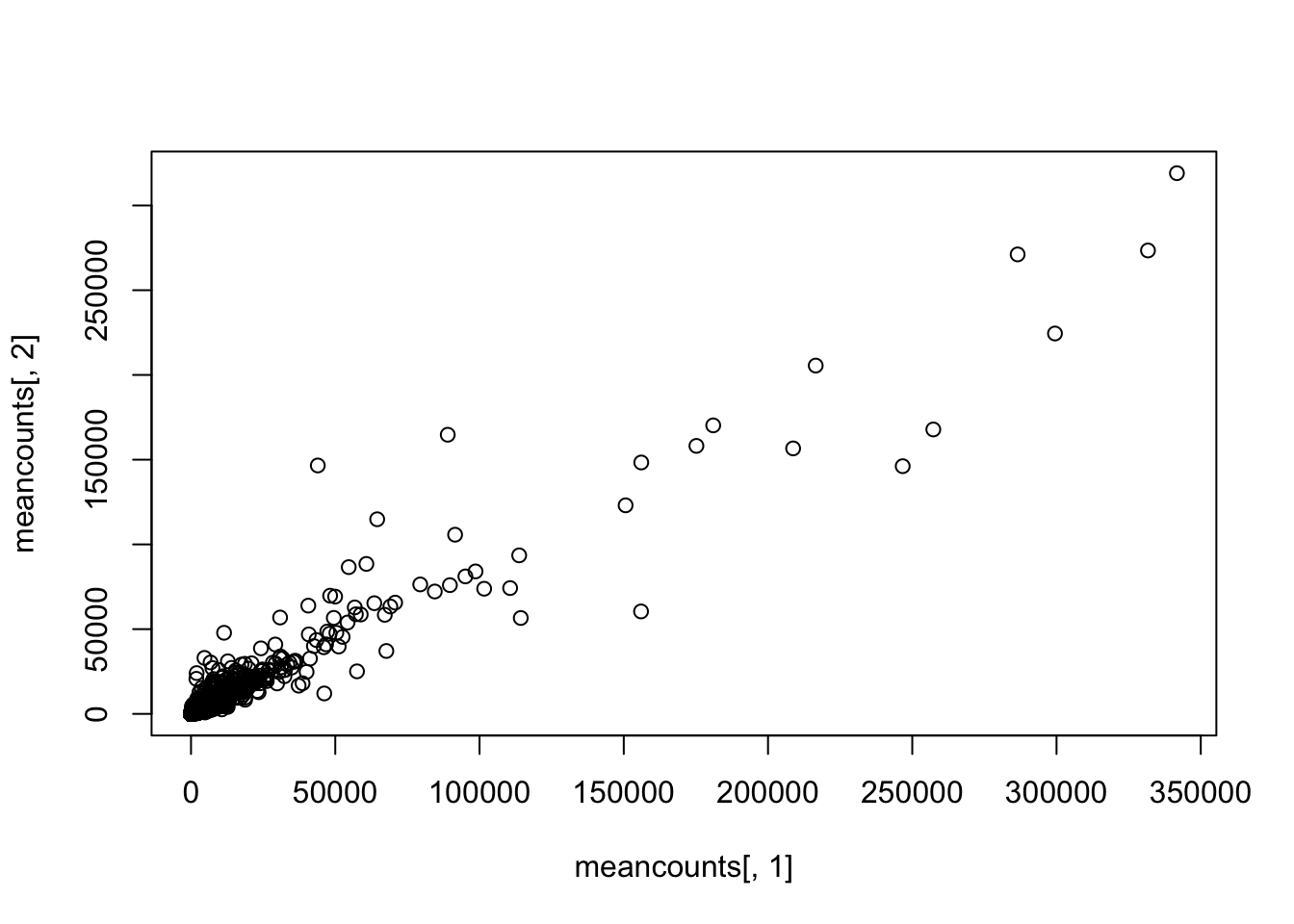
library(ggplot2)

ggplot(meancounts) +
  aes(control.mean, treated.mean) +
  geom_point()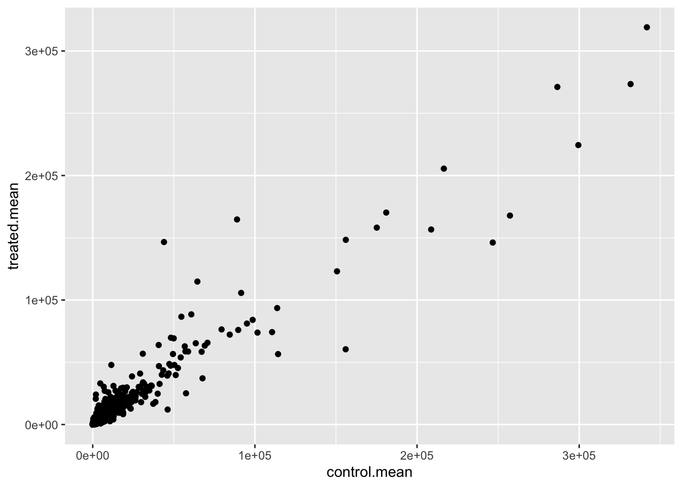
We will make a log-log plot to draw out this skewed data and see what is going on.
plot(meancounts[,1], meancounts[,2], log="xy",
     xlab="log control counts",
     ylab="log of treated counts")
Warning in xy.coords(x, y, xlabel, ylabel, log): 15032 x values <= 0 omitted
from logarithmic plotWarning in xy.coords(x, y, xlabel, ylabel, log): 15281 y values <= 0 omitted
from logarithmic plot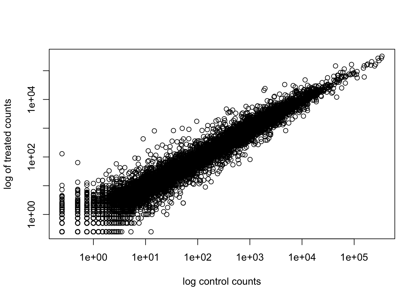
We often log2 transformations when dealing with this sort of data.
log2(20/20)[1] 0log2(40/20)[1] 1log2(20/40)[1] -1log2(80/20)[1] 2This log2 transformation has this nice property where if there is no change the log2 value will be zero and if it double the log2 value will be 1 and if halved it will be -1.
So let’s add a log2 fold change column to our results so far
meancounts$log2fc <- log2( meancounts$treated.mean / meancounts$control.mean )head(meancounts) control.mean treated.mean log2fc
ENSG00000000003 900.75 658.00 -0.45303916
ENSG00000000005 0.00 0.00 NaN
ENSG00000000419 520.50 546.00 0.06900279
ENSG00000000457 339.75 316.50 -0.10226805
ENSG00000000460 97.25 78.75 -0.30441833
ENSG00000000938 0.75 0.00 -InfWe need to get ride of zero count genes that we can not say anything about
zero.values <- which( meancounts[,1:2]==0, arr.ind=TRUE )
to.rm <- unique(zero.values[,1])
mycounts <- meancounts[-to.rm, ]head(mycounts) control.mean treated.mean log2fc
ENSG00000000003 900.75 658.00 -0.45303916
ENSG00000000419 520.50 546.00 0.06900279
ENSG00000000457 339.75 316.50 -0.10226805
ENSG00000000460 97.25 78.75 -0.30441833
ENSG00000000971 5219.00 6687.50 0.35769358
ENSG00000001036 2327.00 1785.75 -0.38194109How many genes are remaining?
nrow(mycounts)[1] 21817Use fold change to see up and down regulated genes.
A common threshold used for calling something differentially expressed is a log2(FoldChange) of greater than 2 or less than -2. Let’s filter the dataset both ways to see how many genes are up or down-regulated.
sum(mycounts$log2fc > 2)[1] 250and down regulated
sum(mycounts$log2fc < -2)[1] 367Do we trust these results? Well not fully because we don’t yet know if these changes are significant…
DESeq2 analysis
Let’s do this the right way. DESeq2 is an R package specifically for analyzing count-based NGS data like RNA-seq. It is available from Bioconductor. Bioconductor is a project to provide tools for analyzing high-throughput genomic data including RNA-seq, ChIP-seq and arrays.
# load up DESeq2
library(DESeq2)
Loading required package: S4VectorsLoading required package: stats4Loading required package: BiocGenericsLoading required package: generics
Attaching package: 'generics'The following objects are masked from 'package:base':
as.difftime, as.factor, as.ordered, intersect, is.element, setdiff,
setequal, union
Attaching package: 'BiocGenerics'The following objects are masked from 'package:stats':
IQR, mad, sd, var, xtabsThe following objects are masked from 'package:base':
anyDuplicated, aperm, append, as.data.frame, basename, cbind,
colnames, dirname, do.call, duplicated, eval, evalq, Filter, Find,
get, grep, grepl, is.unsorted, lapply, Map, mapply, match, mget,
order, paste, pmax, pmax.int, pmin, pmin.int, Position, rank,
rbind, Reduce, rownames, sapply, saveRDS, table, tapply, unique,
unsplit, which.max, which.min
Attaching package: 'S4Vectors'The following object is masked from 'package:utils':
findMatchesThe following objects are masked from 'package:base':
expand.grid, I, unnameLoading required package: IRangesLoading required package: GenomicRangesLoading required package: SeqinfoLoading required package: SummarizedExperimentLoading required package: MatrixGenericsLoading required package: matrixStats
Attaching package: 'MatrixGenerics'The following objects are masked from 'package:matrixStats':
colAlls, colAnyNAs, colAnys, colAvgsPerRowSet, colCollapse,
colCounts, colCummaxs, colCummins, colCumprods, colCumsums,
colDiffs, colIQRDiffs, colIQRs, colLogSumExps, colMadDiffs,
colMads, colMaxs, colMeans2, colMedians, colMins, colOrderStats,
colProds, colQuantiles, colRanges, colRanks, colSdDiffs, colSds,
colSums2, colTabulates, colVarDiffs, colVars, colWeightedMads,
colWeightedMeans, colWeightedMedians, colWeightedSds,
colWeightedVars, rowAlls, rowAnyNAs, rowAnys, rowAvgsPerColSet,
rowCollapse, rowCounts, rowCummaxs, rowCummins, rowCumprods,
rowCumsums, rowDiffs, rowIQRDiffs, rowIQRs, rowLogSumExps,
rowMadDiffs, rowMads, rowMaxs, rowMeans2, rowMedians, rowMins,
rowOrderStats, rowProds, rowQuantiles, rowRanges, rowRanks,
rowSdDiffs, rowSds, rowSums2, rowTabulates, rowVarDiffs, rowVars,
rowWeightedMads, rowWeightedMeans, rowWeightedMedians,
rowWeightedSds, rowWeightedVarsLoading required package: BiobaseWelcome to Bioconductor
Vignettes contain introductory material; view with
'browseVignettes()'. To cite Bioconductor, see
'citation("Biobase")', and for packages 'citation("pkgname")'.
Attaching package: 'Biobase'The following object is masked from 'package:MatrixGenerics':
rowMediansThe following objects are masked from 'package:matrixStats':
anyMissing, rowMediansdds <- DESeqDataSetFromMatrix(countData=counts,
colData=metadata,
design=~dex)converting counts to integer modeWarning in DESeqDataSet(se, design = design, ignoreRank): some variables in
design formula are characters, converting to factorsdds <- DESeq(dds)estimating size factorsestimating dispersionsgene-wise dispersion estimatesmean-dispersion relationshipfinal dispersion estimatesfitting model and testingres <- results(dds)
reslog2 fold change (MLE): dex treated vs control
Wald test p-value: dex treated vs control
DataFrame with 38694 rows and 6 columns
baseMean log2FoldChange lfcSE stat pvalue
<numeric> <numeric> <numeric> <numeric> <numeric>
ENSG00000000003 747.1942 -0.350703 0.168242 -2.084514 0.0371134
ENSG00000000005 0.0000 NA NA NA NA
ENSG00000000419 520.1342 0.206107 0.101042 2.039828 0.0413675
ENSG00000000457 322.6648 0.024527 0.145134 0.168996 0.8658000
ENSG00000000460 87.6826 -0.147143 0.256995 -0.572550 0.5669497
... ... ... ... ... ...
ENSG00000283115 0.000000 NA NA NA NA
ENSG00000283116 0.000000 NA NA NA NA
ENSG00000283119 0.000000 NA NA NA NA
ENSG00000283120 0.974916 -0.66825 1.69441 -0.394385 0.693297
ENSG00000283123 0.000000 NA NA NA NA
padj
<numeric>
ENSG00000000003 0.163017
ENSG00000000005 NA
ENSG00000000419 0.175937
ENSG00000000457 0.961682
ENSG00000000460 0.815805
... ...
ENSG00000283115 NA
ENSG00000283116 NA
ENSG00000283119 NA
ENSG00000283120 NA
ENSG00000283123 NAWe can get some basic summary tallies using the summary() function
summary(res, alpha=0.05)
out of 25258 with nonzero total read count
adjusted p-value < 0.05
LFC > 0 (up)       : 1242, 4.9%
LFC < 0 (down)     : 939, 3.7%
outliers [1]       : 142, 0.56%
low counts [2]     : 9971, 39%
(mean count < 10)
[1] see 'cooksCutoff' argument of ?results
[2] see 'independentFiltering' argument of ?results
Volcano plot
Make a summary plot of our results.
plot(res$log2FoldChange, log(res$padj))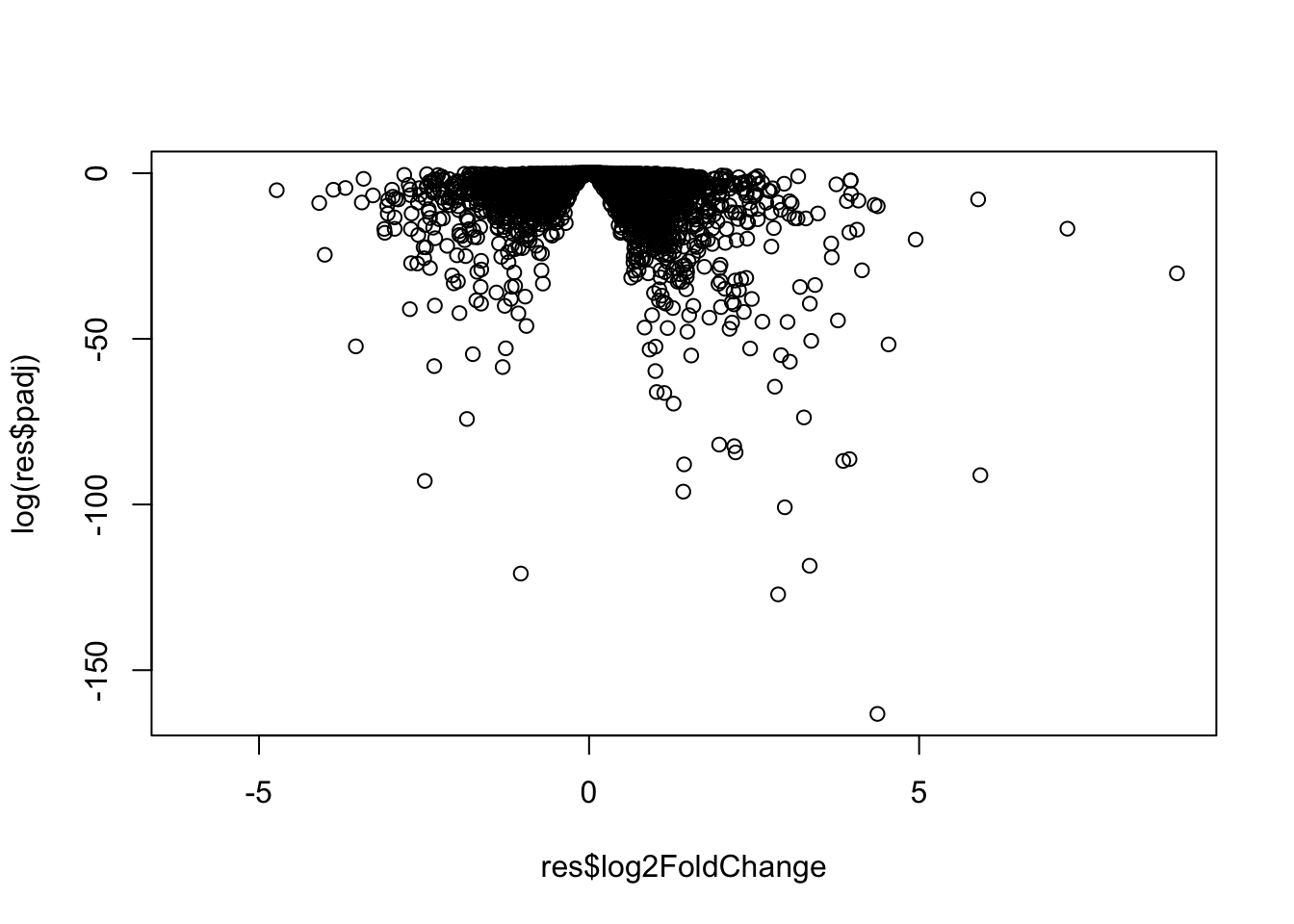
log(0.1)[1] -2.302585log(0.005)[1] -5.298317Finish for today by saving our
Save our results to a CSV file
write.csv(res, file="DESeq2_results.csv")Add annotation data
We need to add missing annotation data to our main res results object. This includes the common gene “symbol”
head(res)log2 fold change (MLE): dex treated vs control
Wald test p-value: dex treated vs control
DataFrame with 6 rows and 6 columns
baseMean log2FoldChange lfcSE stat pvalue
<numeric> <numeric> <numeric> <numeric> <numeric>
ENSG00000000003 747.194195 -0.350703 0.168242 -2.084514 0.0371134
ENSG00000000005 0.000000 NA NA NA NA
ENSG00000000419 520.134160 0.206107 0.101042 2.039828 0.0413675
ENSG00000000457 322.664844 0.024527 0.145134 0.168996 0.8658000
ENSG00000000460 87.682625 -0.147143 0.256995 -0.572550 0.5669497
ENSG00000000938 0.319167 -1.732289 3.493601 -0.495846 0.6200029
padj
<numeric>
ENSG00000000003 0.163017
ENSG00000000005 NA
ENSG00000000419 0.175937
ENSG00000000457 0.961682
ENSG00000000460 0.815805
ENSG00000000938 NAWe will use R and bioconductor to do this “ID mapping”
library("AnnotationDbi")
library("org.Hs.eg.db")
Let’s see what databases we can use for translation/mapping…
columns(org.Hs.eg.db) [1] "ACCNUM" "ALIAS" "ENSEMBL" "ENSEMBLPROT" "ENSEMBLTRANS"
[6] "ENTREZID" "ENZYME" "EVIDENCE" "EVIDENCEALL" "GENENAME"
[11] "GENETYPE" "GO" "GOALL" "IPI" "MAP"
[16] "OMIM" "ONTOLOGY" "ONTOLOGYALL" "PATH" "PFAM"
[21] "PMID" "PROSITE" "REFSEQ" "SYMBOL" "UCSCKG"
[26] "UNIPROT" We can use the mapIds() function now to “translate” between any of these databases.
res$symbol <- mapIds(org.Hs.eg.db,
                     keys=row.names(res), # Our genenames
                     keytype="ENSEMBL",   # Their format
                     column="SYMBOL")     # Format we want
'select()' returned 1:many mapping between keys and columnsQ. Also add “ENTREZID”, “GENENAME” IDs to our
resobject”
res$entres <- mapIds(org.Hs.eg.db,
                     keys=row.names(res), # Our genenames
                     keytype="ENSEMBL",   # Their format
                     column="ENTREZID",
                     multiVals = "list")
'select()' returned 1:many mapping between keys and columnsres$genename <- mapIds(org.Hs.eg.db,
keys=row.names(res), # Our genenames
keytype="ENSEMBL", # Their format
column="GENENAME",
multiVals = "list")'select()' returned 1:many mapping between keys and columnshead(res)log2 fold change (MLE): dex treated vs control
Wald test p-value: dex treated vs control
DataFrame with 6 rows and 9 columns
baseMean log2FoldChange lfcSE stat pvalue
<numeric> <numeric> <numeric> <numeric> <numeric>
ENSG00000000003 747.194195 -0.350703 0.168242 -2.084514 0.0371134
ENSG00000000005 0.000000 NA NA NA NA
ENSG00000000419 520.134160 0.206107 0.101042 2.039828 0.0413675
ENSG00000000457 322.664844 0.024527 0.145134 0.168996 0.8658000
ENSG00000000460 87.682625 -0.147143 0.256995 -0.572550 0.5669497
ENSG00000000938 0.319167 -1.732289 3.493601 -0.495846 0.6200029
padj symbol entres genename
<numeric> <character> <list> <list>
ENSG00000000003 0.163017 TSPAN6 7105 tetraspanin 6
ENSG00000000005 NA TNMD 64102 tenomodulin
ENSG00000000419 0.175937 DPM1 8813 dolichyl-phosphate m..
ENSG00000000457 0.961682 SCYL3 57147 SCY1 like pseudokina..
ENSG00000000460 0.815805 FIRRM 55732 FIGNL1 interacting r..
ENSG00000000938 NA FGR 2268 FGR proto-oncogene, ..Pathway analysis
What known biological pathways do our differentially expressed genes overlap with (i.e. play a role in)?
There are lot’s of bioconductor packages to do this type of analysis.
We will use one of the oldest called gage along with pathview to render ncice pics of the pathways we find.
We can install these with the command: BiocManager::install( c("pathview", "gage", "gageData") )
library(pathview)
library(gage)
library(gageData)
Have a wee peek what is in gageData
# Examine the first 2 pathways in this kegg set for humans
data(kegg.sets.hs)
head(kegg.sets.hs, 2)
$`hsa00232 Caffeine metabolism`
[1] "10" "1544" "1548" "1549" "1553" "7498" "9"
$`hsa00983 Drug metabolism - other enzymes`
[1] "10" "1066" "10720" "10941" "151531" "1548" "1549" "1551"
[9] "1553" "1576" "1577" "1806" "1807" "1890" "221223" "2990"
[17] "3251" "3614" "3615" "3704" "51733" "54490" "54575" "54576"
[25] "54577" "54578" "54579" "54600" "54657" "54658" "54659" "54963"
[33] "574537" "64816" "7083" "7084" "7172" "7363" "7364" "7365"
[41] "7366" "7367" "7371" "7372" "7378" "7498" "79799" "83549"
[49] "8824" "8833" "9" "978" The main gage() function that does the work wants a simple vector as input.
foldchanges = res$log2FoldChange
names(foldchanges) = res$symbol
head(foldchanges)
TSPAN6 TNMD DPM1 SCYL3 FIRRM FGR
-0.35070296 NA 0.20610728 0.02452701 -0.14714263 -1.73228897 The KEGG database uses ENTREZ ids so we need to provide these in our input vector for gage:
names(foldchanges) <- res$entresNow we can run gage()
# Get the results
keggres = gage(foldchanges, gsets=kegg.sets.hs)
What is in the output object keggres
attributes(keggres)$names
[1] "greater" "less" "stats" # Look at the first three down (less) pathways
head(keggres$less, 3) p.geomean stat.mean p.val
hsa05332 Graft-versus-host disease 0.0004250607 -3.473335 0.0004250607
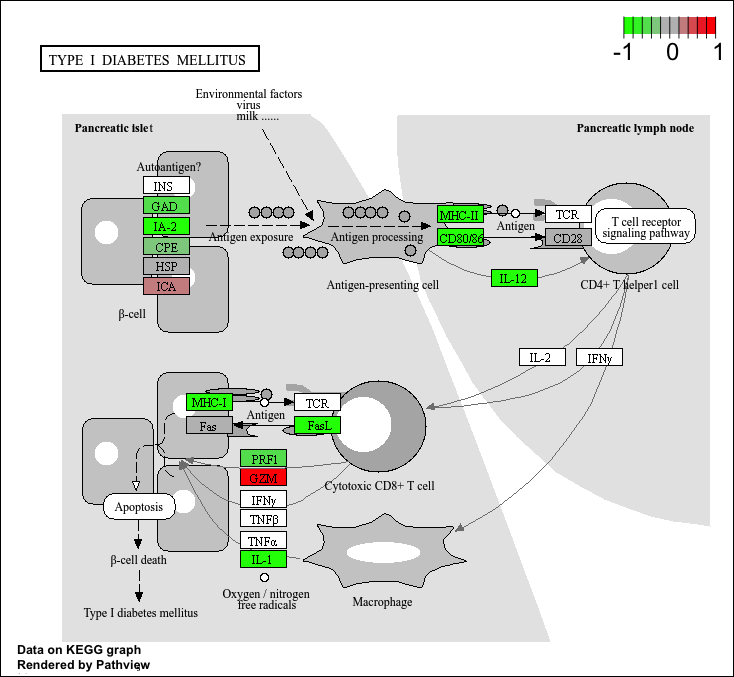
hsa04940 Type I diabetes mellitus 0.0017820379 -3.002350 0.0017820379
hsa05310 Asthma 0.0020046180 -3.009045 0.0020046180
q.val set.size exp1
hsa05332 Graft-versus-host disease 0.09053792 40 0.0004250607
hsa04940 Type I diabetes mellitus 0.14232788 42 0.0017820379
hsa05310 Asthma 0.14232788 29 0.0020046180We can use the pathview function to render a figure of any of these pathways along with annotation for our DEGs
Let’s see the hsa05310 Asthma pathway with our DEGs colored up:
pathview(gene.data=foldchanges, pathway.id="hsa05310")'select()' returned 1:1 mapping between keys and columnsInfo: Working in directory /Users/yanelee/Downloads/BIMM143/class13/class13labInfo: Writing image file hsa05310.pathview.png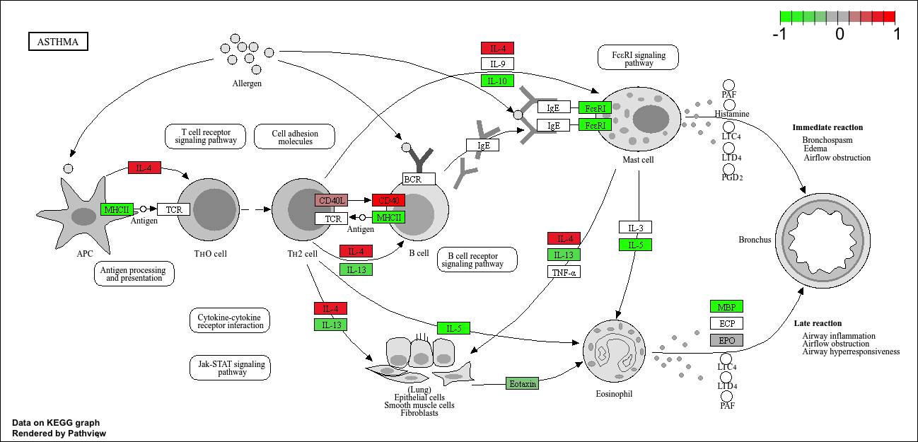
Q. Can you render and insert here the pathway figure for “Graft-versus-host disease” and “Type I diabetes”?
For “Graft-versus-host-disease”…
pathview(gene.data=foldchanges, pathway.id="hsa05332")'select()' returned 1:1 mapping between keys and columnsInfo: Working in directory /Users/yanelee/Downloads/BIMM143/class13/class13labInfo: Writing image file hsa05332.pathview.png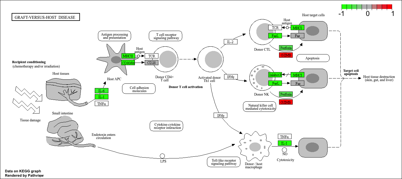
For “Type 1 diabetes”…
pathview(gene.data=foldchanges, pathway.id="hsa04940")'select()' returned 1:1 mapping between keys and columnsInfo: Working in directory /Users/yanelee/Downloads/BIMM143/class13/class13labInfo: Writing image file hsa04940.pathview.png