Yane's Site
My classwork from BIMM143
Class 17: Analyzing Sequencing Data
Yane Lee PID A17670350
Downstream Analysis
With each sample having its own directory containing the Kallisto output, we can import the transcript count estimates into R using:
if (!requireNamespace("BiocManager", quietly = TRUE))
    install.packages("BiocManager")

BiocManager::install("rhdf5")
Bioconductor version 3.22 (BiocManager 1.30.27), R 4.5.2 (2025-10-31)

Warning: package(s) not installed when version(s) same as or greater than current; use
  `force = TRUE` to re-install: 'rhdf5'
library(tximport)

folders <- dir(pattern="SRR21568*")
samples <- sub("_quant","",folders)
files <- file.path(folders, "abundance.h5")
names(files) <- samples

txi.kallisto <- tximport(files, type="kallisto", txOut=TRUE)
1 2 3 4
head(txi.kallisto$counts)
                SRR2156848 SRR2156849 SRR2156850 SRR2156851
ENST00000539570          0          0    0.00000          0
ENST00000576455          0          0    2.62037          0
ENST00000510508          0          0    0.00000          0
ENST00000474471          0          1    1.00000          0
ENST00000381700          0          0    0.00000          0
ENST00000445946          0          0    0.00000          0
We now have our estimated transcript counts for each sample in R. We can see how many transcripts we have for each sample:
colSums(txi.kallisto$counts)
SRR2156848 SRR2156849 SRR2156850 SRR2156851
   2563611    2600800    2372309    2111474
And how many transcripts are detected in at least one sample:
sum(rowSums(txi.kallisto$counts)>0)
[1] 94561
We want to filter out the annotated transcripts with no reads
to.keep <- rowSums(txi.kallisto$counts) > 0
kset.nonzero <- txi.kallisto$counts[to.keep,]
keep2 <- apply(kset.nonzero,1,sd)>0
x <- kset.nonzero[keep2,]
Principal Component Analysis
We can now apply any exploratory analysis technique to this counts matrix. As an example, we will perform a PCA of the transcriptomic profiles of these samples.
pca <- prcomp(t(x), scale=TRUE)
summary(pca)
Importance of components:
                            PC1      PC2      PC3   PC4
Standard deviation     183.6379 177.3605 171.3020 1e+00
Proportion of Variance   0.3568   0.3328   0.3104 1e-05
Cumulative Proportion    0.3568   0.6895   1.0000 1e+00
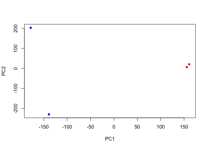
Now we can use the first two principal components as a co-ordinate system for visualizing the summarized transcriptomic profiles of each sample:
plot(pca$x[,1], pca$x[,2],
     col=c("blue","blue","red","red"),
     xlab="PC1", ylab="PC2", pch=16)
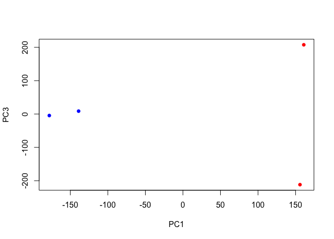
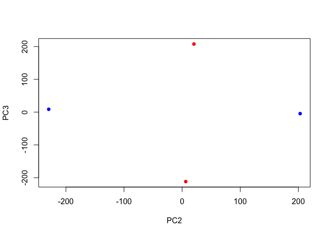
Q. Q. Use ggplot to make a similar figure of PC1 vs PC2 and a separate figure PC1 vs PC3 and PC2 vs PC3.
plot(pca$x[,1], pca$x[,3],
     col=c("blue","blue","red","red"),
     xlab="PC1", ylab="PC3", pch=16)
plot(pca$x[,2], pca$x[,3],
     col=c("blue","blue","red","red"),
     xlab="PC2", ylab="PC3", pch=16)
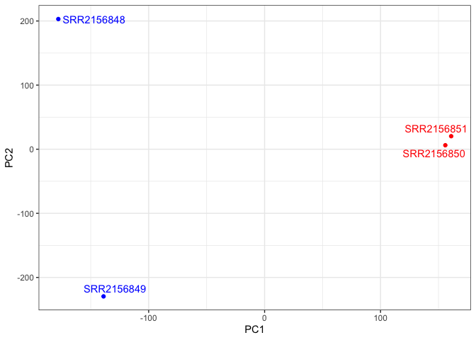
Plot with labels for the two control samples (SRR2156848 and SRR2156849) and the two enhancer-targeting CRISPR-Cas9 samples (SRR2156850 and SRR2156851).
library(ggplot2)
library(ggrepel)

mycols <- c("blue","blue","red","red")

ggplot(pca$x) +
  aes(PC1, PC2, label=rownames(pca$x)) +
  geom_point( col=mycols ) +
  geom_text_repel( col=mycols ) +
  theme_bw()
Differential-expression analysis
We can use DESeq2 to complete the differential-expression analysis that we are already familiar with:
library(DESeq2)
Loading required package: S4Vectors

Loading required package: stats4

Loading required package: BiocGenerics

Loading required package: generics


Attaching package: 'generics'

The following objects are masked from 'package:base':

    as.difftime, as.factor, as.ordered, intersect, is.element, setdiff,
    setequal, union


Attaching package: 'BiocGenerics'

The following objects are masked from 'package:stats':

    IQR, mad, sd, var, xtabs

The following objects are masked from 'package:base':

    anyDuplicated, aperm, append, as.data.frame, basename, cbind,
    colnames, dirname, do.call, duplicated, eval, evalq, Filter, Find,
    get, grep, grepl, is.unsorted, lapply, Map, mapply, match, mget,
    order, paste, pmax, pmax.int, pmin, pmin.int, Position, rank,
    rbind, Reduce, rownames, sapply, saveRDS, table, tapply, unique,
    unsplit, which.max, which.min


Attaching package: 'S4Vectors'

The following object is masked from 'package:utils':

    findMatches

The following objects are masked from 'package:base':

    expand.grid, I, unname

Loading required package: IRanges

Loading required package: GenomicRanges

Loading required package: Seqinfo

Loading required package: SummarizedExperiment

Loading required package: MatrixGenerics

Loading required package: matrixStats


Attaching package: 'MatrixGenerics'

The following objects are masked from 'package:matrixStats':

    colAlls, colAnyNAs, colAnys, colAvgsPerRowSet, colCollapse,
    colCounts, colCummaxs, colCummins, colCumprods, colCumsums,
    colDiffs, colIQRDiffs, colIQRs, colLogSumExps, colMadDiffs,
    colMads, colMaxs, colMeans2, colMedians, colMins, colOrderStats,
    colProds, colQuantiles, colRanges, colRanks, colSdDiffs, colSds,
    colSums2, colTabulates, colVarDiffs, colVars, colWeightedMads,
    colWeightedMeans, colWeightedMedians, colWeightedSds,
    colWeightedVars, rowAlls, rowAnyNAs, rowAnys, rowAvgsPerColSet,
    rowCollapse, rowCounts, rowCummaxs, rowCummins, rowCumprods,
    rowCumsums, rowDiffs, rowIQRDiffs, rowIQRs, rowLogSumExps,
    rowMadDiffs, rowMads, rowMaxs, rowMeans2, rowMedians, rowMins,
    rowOrderStats, rowProds, rowQuantiles, rowRanges, rowRanks,
    rowSdDiffs, rowSds, rowSums2, rowTabulates, rowVarDiffs, rowVars,
    rowWeightedMads, rowWeightedMeans, rowWeightedMedians,
    rowWeightedSds, rowWeightedVars

Loading required package: Biobase

Welcome to Bioconductor

    Vignettes contain introductory material; view with
    'browseVignettes()'. To cite Bioconductor, see
    'citation("Biobase")', and for packages 'citation("pkgname")'.


Attaching package: 'Biobase'

The following object is masked from 'package:MatrixGenerics':

    rowMedians

The following objects are masked from 'package:matrixStats':

    anyMissing, rowMedians
sampleTable <- data.frame(condition = factor(rep(c("control", "treatment"), each = 2)))
rownames(sampleTable) <- colnames(txi.kallisto$counts)
dds <- DESeqDataSetFromTximport(txi.kallisto,
                                sampleTable,
                                ~condition)
using counts and average transcript lengths from tximport
dds <- DESeq(dds)
estimating size factors

using 'avgTxLength' from assays(dds), correcting for library size

estimating dispersions

gene-wise dispersion estimates

mean-dispersion relationship

-- note: fitType='parametric', but the dispersion trend was not well captured by the
   function: y = a/x + b, and a local regression fit was automatically substituted.
   specify fitType='local' or 'mean' to avoid this message next time.

final dispersion estimates

fitting model and testing
res <- results(dds)
head(res)
log2 fold change (MLE): condition treatment vs control
Wald test p-value: condition treatment vs control
DataFrame with 6 rows and 6 columns
                 baseMean log2FoldChange     lfcSE      stat    pvalue
                <numeric>      <numeric> <numeric> <numeric> <numeric>
ENST00000539570  0.000000             NA        NA        NA        NA
ENST00000576455  0.761453       3.155061   4.86052 0.6491203  0.516261
ENST00000510508  0.000000             NA        NA        NA        NA
ENST00000474471  0.484938       0.181923   4.24871 0.0428185  0.965846
ENST00000381700  0.000000             NA        NA        NA        NA
ENST00000445946  0.000000             NA        NA        NA        NA
                     padj
                <numeric>
ENST00000539570        NA
ENST00000576455        NA
ENST00000510508        NA
ENST00000474471        NA
ENST00000381700        NA
ENST00000445946        NA